一 : 51插值与拟合例题
1 山区地貌:在某山区测得一些地点的高程如下表:(平面区域1200<=x<=4000,1200<=y<=3600),试作出该山区的地貌图和等高线图,并对几种插值方法进行比较。
2 用给定的多项式,如y=x3-6x2+5x-3,产生一组数据(xi,yi,i=1,2,…,n),再在yi上添加随机干扰(可用rand产生(0,1)均匀分布随机数,或用rands产生N(0,1)分布随机数),然后用xi和添加了随机干扰的yi作的3次多项式拟合,与原系数比较。如果作2或4次多项式拟合,结果如何?
3 用电压V=10伏的电池给电容器充电,电容器上t时刻的电压为 ,其中V0是电容器的初始电压, 是充电常数。试由下面一组t,V数据确定V0, 。
2用给定的多项式,如y=x3-6x2+5x-3,产生一组数据(xi,yi,i=1,2,…,n),再在yi上添加随机干扰(可用rand产生(0,1)均匀分布随机数,或用rands产生N(0,1)分布随机数),然后用xi和添加了随机干扰的yi作的3次多项式拟合,与原系数比较。
分别作1、2、4、6次多项式拟合,比较结果,体会欠拟合、过拟合现象。
解:程序如下:
x=1:0.5:10;
y=x.^3-6*x.^2+5*x-3;
y0=y+rand;
f1=polyfit(x,y0,1)%输出多项式系数
y1=polyval(f1,x);%计算各x点的拟合值
plot(x,y,'+',x,y1)
grid on
title('一次拟合曲线');
figure(2);
f2=polyfit(x,y0,2)%2次多项式拟合
y2=polyval(f2,x);
plot(x,y,'+',x,y2);
grid on
title('二次拟合曲线');
figure(3);
f4=polyfit(x,y0,4)%4次多项式拟合
y3=polyval(f4,x);
plot(x,y,'+',x,y3)
grid on
title('四次拟合曲线');
figure(4);
f6=polyfit(x,y0,6)%6次多项式拟合
y4=polyval(f6,x);
plot(x,y,'+',x,y4)
grid on
title('六次拟合曲线');
运行结果如下:依次为各个拟合曲线的系数(按降幂排列)
f1 =43.2000 -149.0663
f2 = 10.5000 -72.3000 89.8087
f4 =0.0000 1.0000 -6.0000 5.0000 -2.5913
f6 = 0.0000 -0.0000 0.0000 1.0000 -6.0000 5.0000 -2.4199
运行后,比较拟合后多项式和原式的系数,发现四次多项式系数与原系数比较接近,四次多项式的四次项系数很小。作图后,发现一次和二次多项式的图形与原函数的差别比较大,属于欠拟合的情况,而四次多项式和六次多项式符合得比较好。作图如下:
3.解:据题意分析如下:电容器充电的数学模型已经建立。v(t)?V?(V?V0)exp(?t/?)(已知V=10)可见,v(t)与τ成指数变化关系,所以在通过曲线拟合的时候,使用指数曲线y=a1eax。(非线性拟合)。首先进行变量2
代换在程序中用v1代替v(t),t0代替τ,v2是拟合后的曲线方程:
对v(t)?10?(10?v0)exp(?t/?)变形后取对数,有ln(10?v(t))?ln(10?v0)?(?t/?) 令y=ln(10-v(t)) ,f1=ln(10-?0) ,f2= -1/t0,则
v0=10-exp(f(2)), t0= -1/ f(1)。
编写程序如下:
51插值与拟合例题_拟合值
t=[0.5 1 2 3 4 5 7 9];
v1=[6.36 6.48 7.26 8.22 8.66 8.99 9.43 9.63]; y=log(10- v1); f=polyfit(t,y,1) t0=-1/f(1)
v0=10-exp(f(2))
v2=10-(10-v0)*exp(-t/t0); plot(t,v1,'rx',t,v2,'k:') grid on
xlabel('时间t(s)'),ylabel('充电电压(V)'); title('电容器充电电压与时间t的曲线');
程序运行输出结果如下: f =-0.2835 1.4766
t0 = 3.5269 v0 =5.6221
即电容器的初始电压为 v0 =5.6221,τ=3.5629。
4.某年美国旧车价格的调查资料如下表其中xi表示轿车的使用年数,yi表示相应的平均价格。试分析用什么形式的曲线来拟合上述的数据,并预测使用4.5年后轿车的平均价格大致
为多少?
yi
538
484
290
226
204
2615 1943 1494 1087 765
5 汽车制造厂生产的某种轿车的外形数据如下表所示
试找出最佳的拟合曲线拟合以上数据
51插值与拟合例题_拟合值
6
二 : 拟合值与残差

拟合值 拟合值与残差

拟合值 拟合值与残差

拟合值 拟合值与残差
拟合值 拟合值与残差

拟合值 拟合值与残差
拟合值 拟合值与残差
拟合值 拟合值与残差
拟合值 拟合值与残差
拟合值 拟合值与残差
拟合值 拟合值与残差
拟合值 拟合值与残差
拟合值 拟合值与残差
拟合值 拟合值与残差
拟合值 拟合值与残差
拟合值 拟合值与残差
拟合值 拟合值与残差
拟合值 拟合值与残差
拟合值 拟合值与残差
拟合值 拟合值与残差

拟合值 拟合值与残差

拟合值 拟合值与残差
拟合值 拟合值与残差
拟合值 拟合值与残差
拟合值 拟合值与残差
拟合值 拟合值与残差
拟合值 拟合值与残差

拟合值 拟合值与残差
拟合值 拟合值与残差

拟合值 拟合值与残差
拟合值 拟合值与残差
拟合值 拟合值与残差
拟合值 拟合值与残差
拟合值 拟合值与残差
拟合值 拟合值与残差
拟合值 拟合值与残差
拟合值 拟合值与残差
拟合值 拟合值与残差
拟合值 拟合值与残差
拟合值 拟合值与残差

拟合值 拟合值与残差
拟合值 拟合值与残差
拟合值 拟合值与残差

三 : 拟合值与残差
Analysis of Cross Section and Panel Data
Yan Zhang School of Economics, Fudan University CCER, Fudan University
Introductory Econometrics
A Modern Approach
Yan Zhang School of Economics, Fudan University CCER, Fudan University
Analysis of Cross Section and Panel Data
Part 1. Regression Analysis on Cross Sectional Data
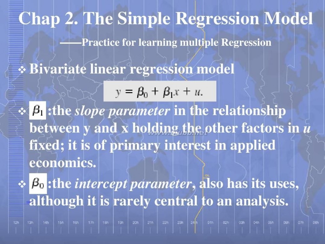
Chap 2. The Simple Regression Model
——Practice for learning multiple Regression
Bivariate linear regression model :the slope parameter in the relationship between y and x holding the other factors in u fixed; it is of primary interest in applied economics. :the intercept parameter, also has its uses, although it is rarely central to an analysis.
More Discussion
:A one-unit change in x has the same effect on y, regardless of the initial value of x.
Increasing returns: wage-education (f. form)
Can we draw ceteris paribus conclusions about how x affects y from a random sample of data, when we are ignoring all the other factors?
Only if we make an assumption restricting how the unobservable random variable u is related to the explanatory variable x
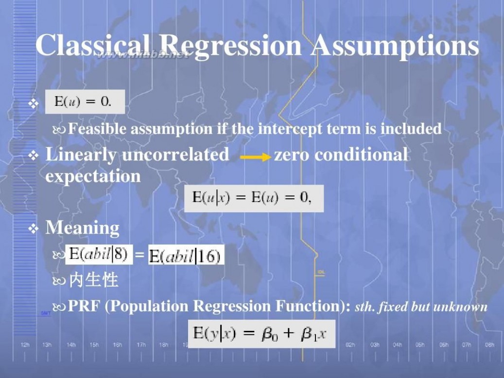
Classical Regression Assumptions
Feasible assumption if the intercept term is included
Linearly uncorrelated expectation Meaning
= 内生性
zero conditional
PRF (Population Regression Function): sth. fixed but unknown
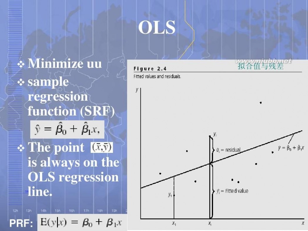
OLS
Minimize uu sample regression function (SRF) The point is always on the OLS regression line.
PRF:
拟合值与残差
OLS
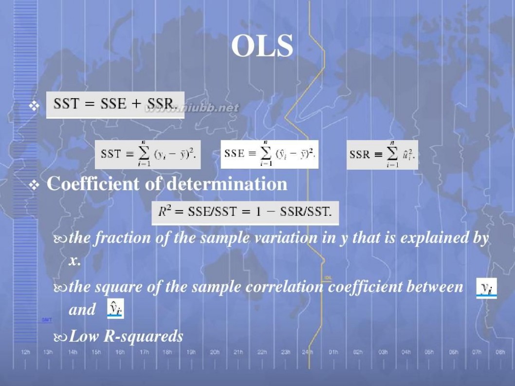
Coefficient of determination
the fraction of the sample variation in y that is explained by x. the square of the sample correlation coefficient between and Low R-squareds
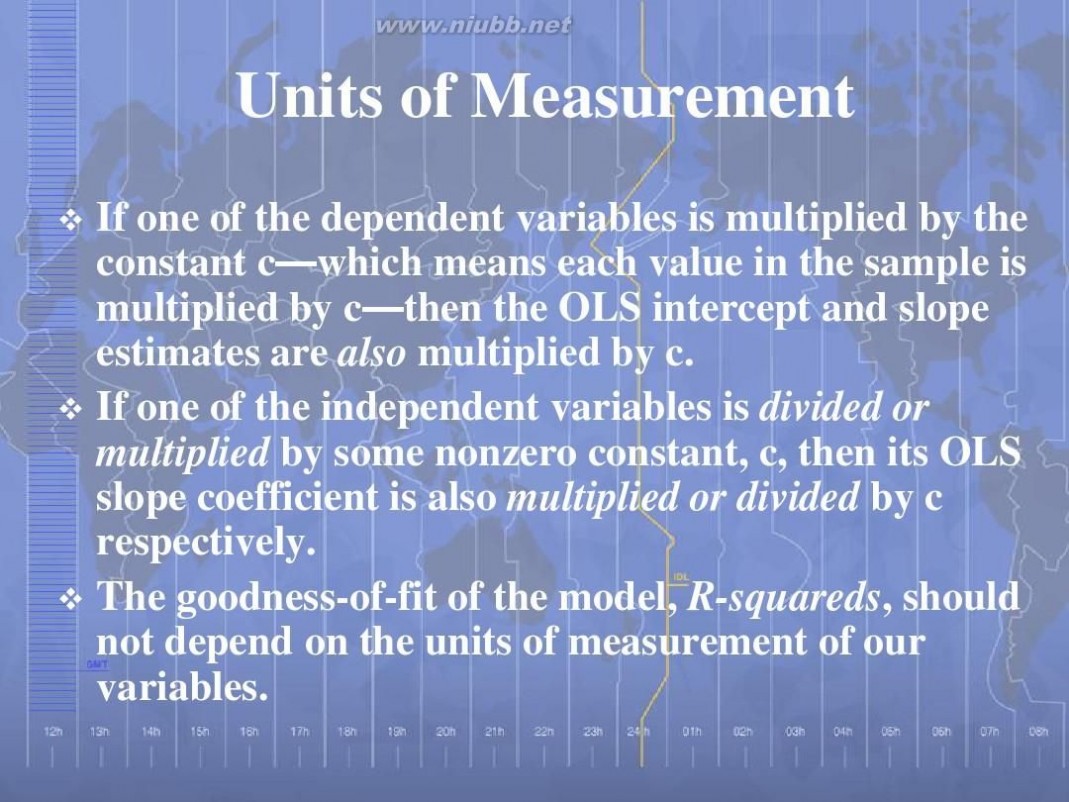
Units of Measurement
If one of the dependent variables is multiplied by the constant c—which means each value in the sample is multiplied by c—then the OLS intercept and slope estimates are also multiplied by c. If one of the independent variables is divided or multiplied by some nonzero constant, c, then its OLS slope coefficient is also multiplied or divided by c respectively. The goodness-of-fit of the model, R-squareds, should not depend on the units of measurement of our variables.
Function Form
Linear Nonlinear Logarithmic dependent variable
A Percentage change in y, semi-elasticity an increasing return to edu. Other nonlinearity: diploma effect
Bi-Logarithmic
A a Constant elasticity
Bi-Logarithmic
A a Constant elasticity
Change of units of measurement
P45, error: b0*=b0+log(c1)-b1log(c2) =
Change of units of measurement
P45, error b0*=b0+log(c1)-b1log(c2 =
Be proficient at interpreting the coef.
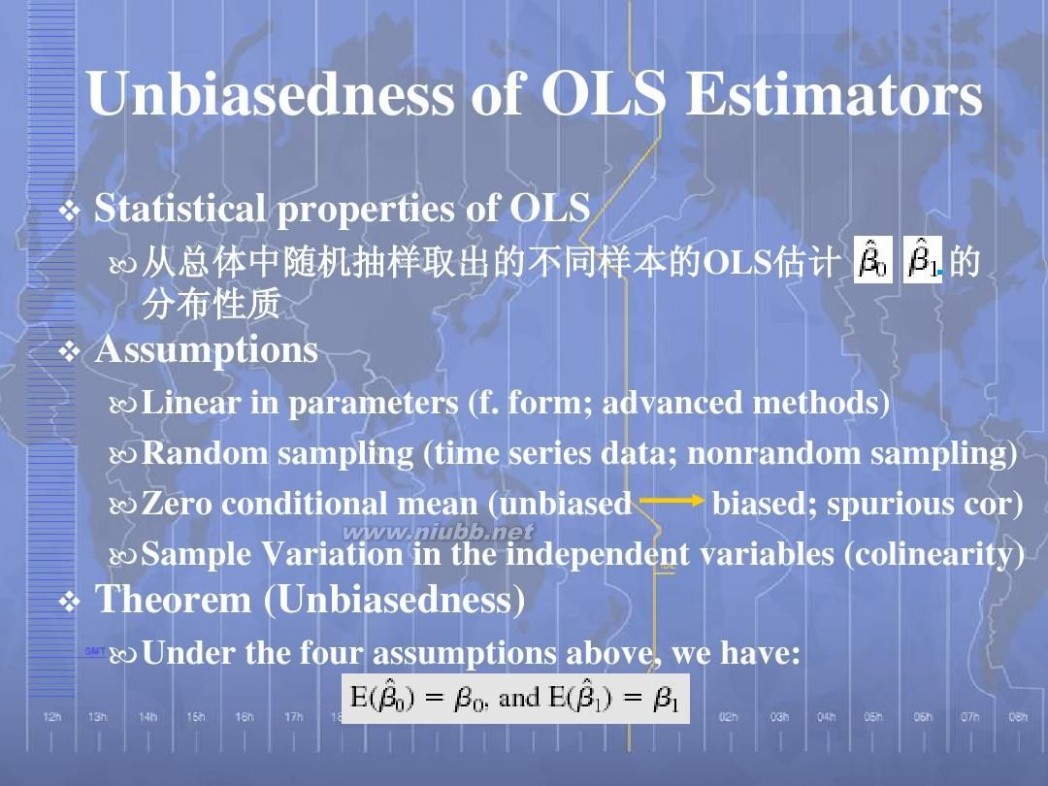
Unbiasedness of OLS Estimators
Statistical properties of OLS
从总体中随机抽样取出的不同样本的OLS估计 估计 从总体中随机抽样取出的不同样本的 分布性质 的
Assumptions
Linear in parameters (f. form; advanced methods) Random sampling (time series data; nonrandom sampling) Zero conditional mean (unbiased biased; spurious cor) Sample Variation in the independent variables (colinearity)
Theorem (Unbiasedness)
Under the four assumptions above, we have:
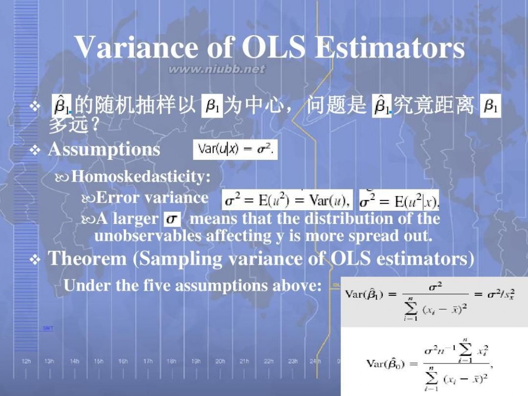
Variance of OLS Estimators
的随机抽样以 多远? 多远? Assumptions 为中心,问题是 为中心, 究竟距离
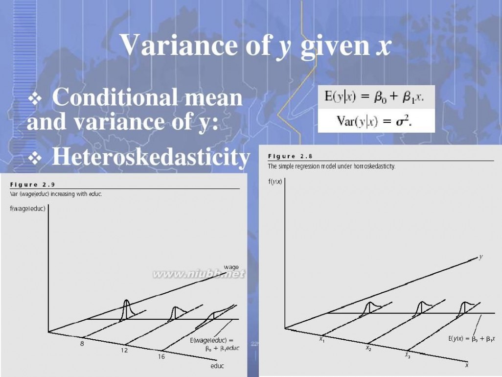
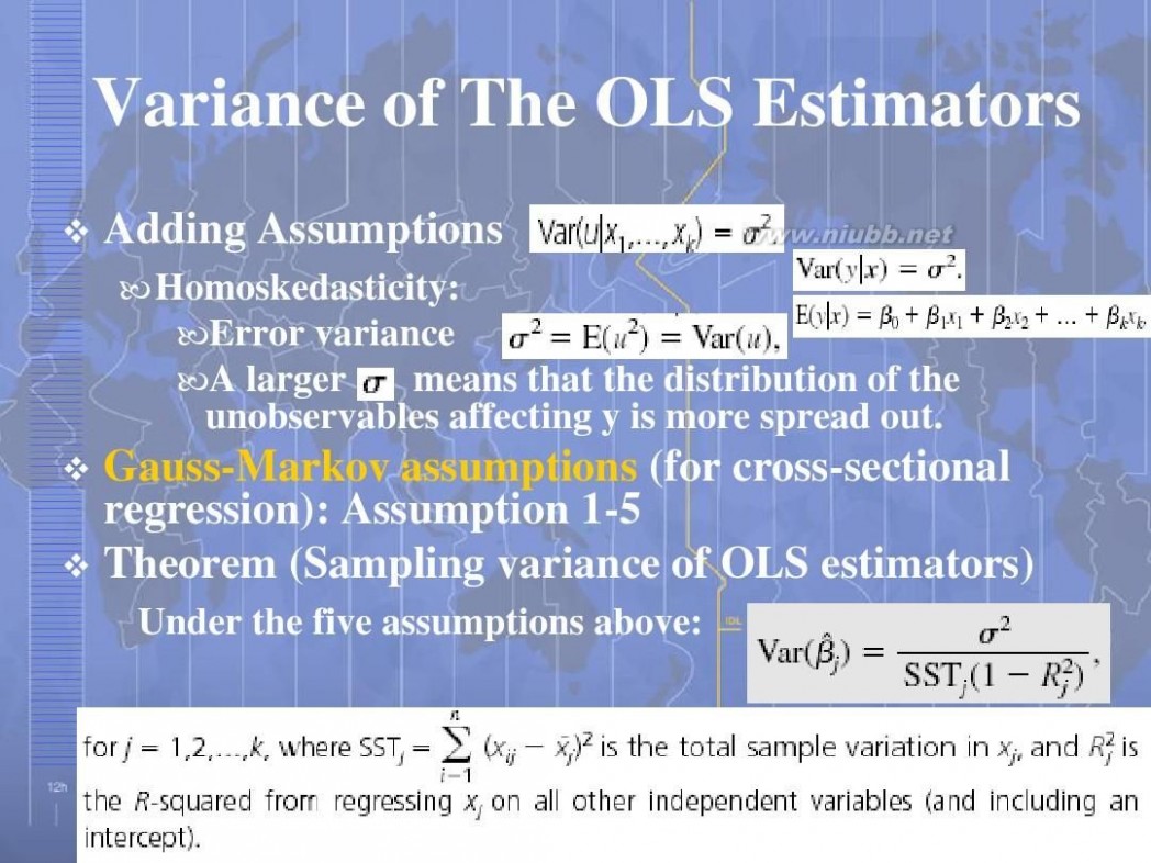
Homoskedasticity: Error variance A larger means that the distribution of the unobservables affecting y is more spread out.
Theorem (Sampling variance of OLS estimators)
Under the five assumptions above:
Variance of y given x
Conditional mean and variance of y: Heteroskedasticity
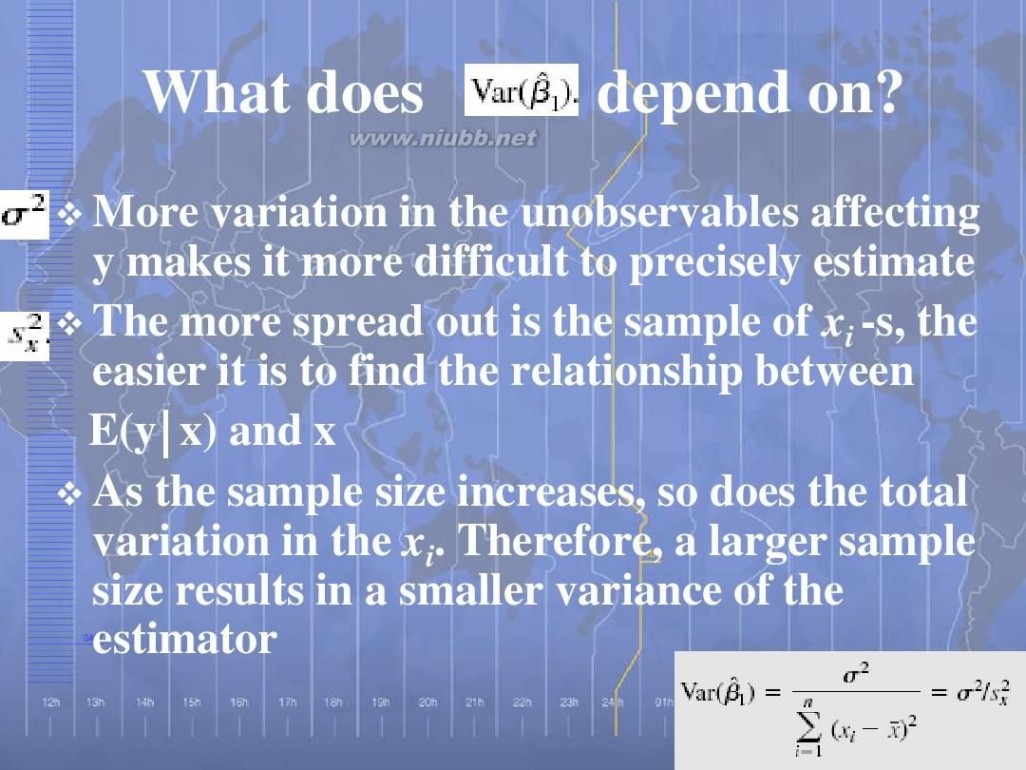
What does
depend on?
More variation in the unobservables affecting y makes it more difficult to precisely estimate The more spread out is the sample of xi -s, the easier it is to find the relationship between E(y x) and x As the sample size increases, so does the total variation in the xi. Therefore, a larger sample size results in a smaller variance of the estimator
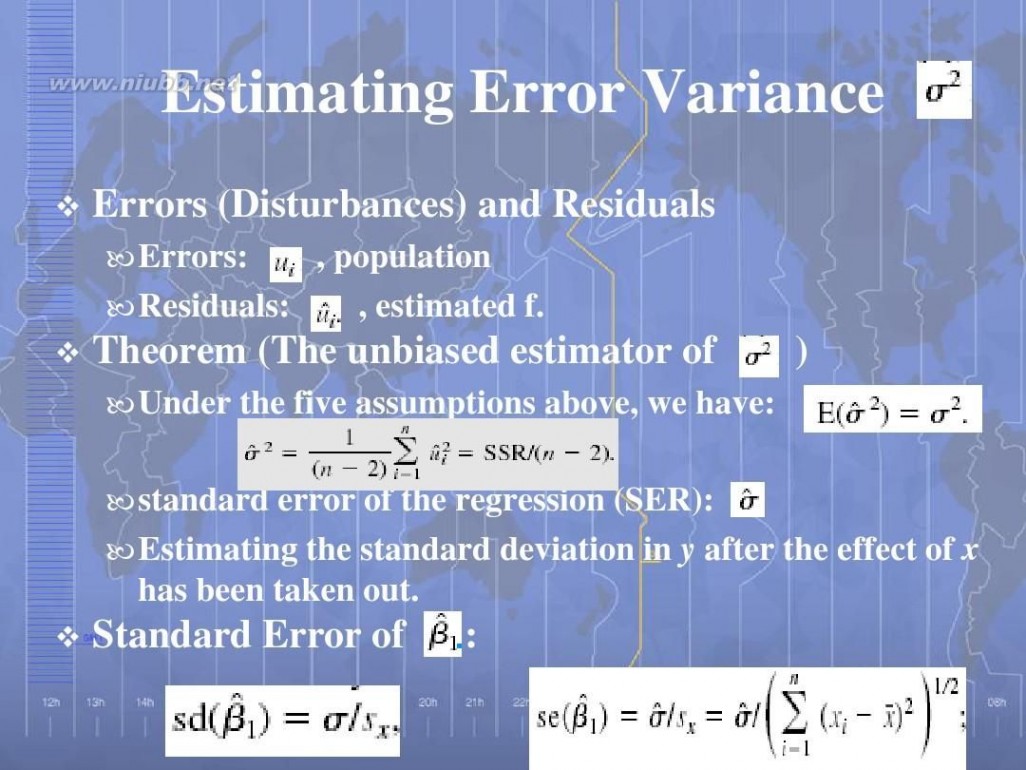
Estimating Error Variance
Errors (Disturbances) and Residuals
Errors: , population Residuals: , estimated f.
Theorem (The unbiased estimator of
Under the five assumptions above, we have:
)
standard error of the regression (SER): Estimating the standard deviation in y after the effect of x has been taken out.
Standard Error of
:
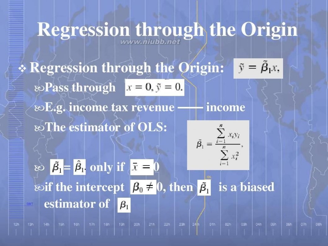
Regression through the Origin
Regression through the Origin:
Pass through E.g. income tax revenue —— income The estimator of OLS: = only if 0 0, then is a biased
if the intercept estimator of
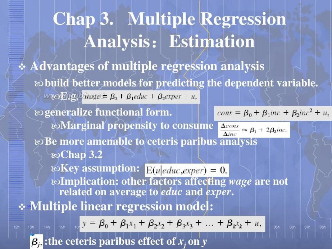
Chap 3. Multiple Regression Analysis:Estimation :
Advantages of multiple regression analysis
build better models for predicting the dependent variable. E.g. generalize functional form. Marginal propensity to consume Be more amenable to ceteris paribus analysis Chap 3.2 Key assumption: Implication: other factors affecting wage are not related on average to educ and exper.
Multiple linear regression model:
:the ceteris paribus effect of xj on y
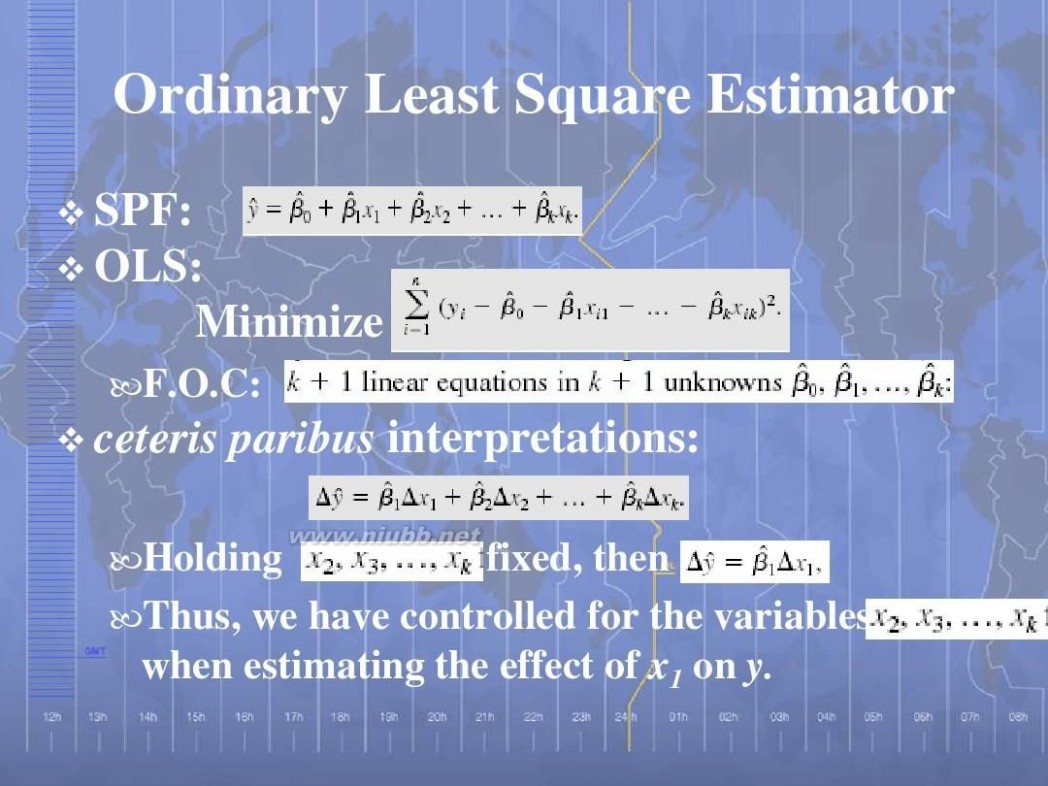
Ordinary Least Square Estimator
SPF: OLS: Minimize
F.O.C:
ceteris paribus interpretations:
Holding fixed, then Thus, we have controlled for the variables when estimating the effect of x1 on y.
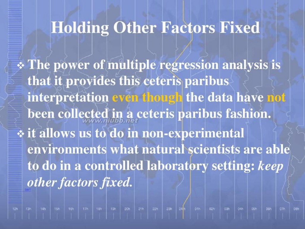
Holding Other Factors Fixed
The power of multiple regression analysis is that it provides this ceteris paribus interpretation even though the data have not been collected in a ceteris paribus fashion. it allows us to do in non-experimental environments what natural scientists are able to do in a controlled laboratory setting: keep other factors fixed.
OLS and Ceteris Paribus Effects
Step of OLS:
(1) (2) :the OLS residuals from a multiple regression of x1 on :the OLS estimator from a simple regression of y on
measures the effect of x1 on y after x2,…, xk have been partialled or netted out. Two special cases in which the simple regression of y on x1 will produce the same OLS estimate on x1 as the regression of y on x1 and x2.
Goodness-of-fit
also equal the squared correlation coef. between the actual and the fitted values of y. R never decreases, and it usually increases when another independent variable is added to a regression. The factor that should determine
whether an explanatory variable belongs in a model is whether the explanatory variable has a nonzero partial effect on y in the population.
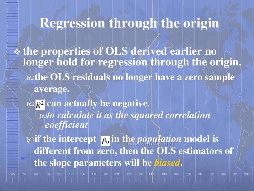
Regression through the origin
the properties of OLS derived earlier no longer hold for regression through the origin.
the OLS residuals no longer have a zero sample average. can actually be negative. to calculate it as the squared correlation coefficient if the intercept in the population model is different from zero, then the OLS estimators of the slope parameters will be biased.
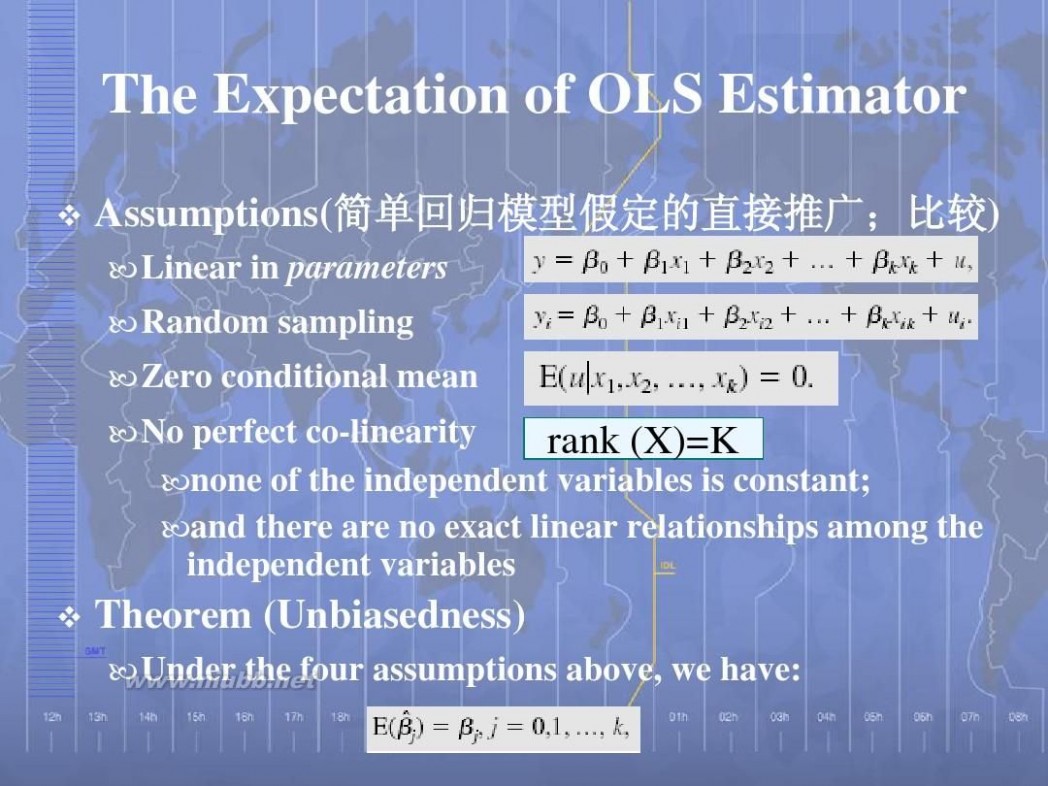
The Expectation of OLS Estimator
Assumptions(简单回归模型假定的直接推广;比较) 简单回归模型假定的直接推广;比较 简单回归模型假定的直接推广
Linear in parameters Random sampling Zero conditional mean No perfect co-linearity rank (X)=K none of the independent variables is constant; and there are no exact linear relationships among the independent variables
Theorem (Unbiasedness)
Under the four assumptions above, we have:
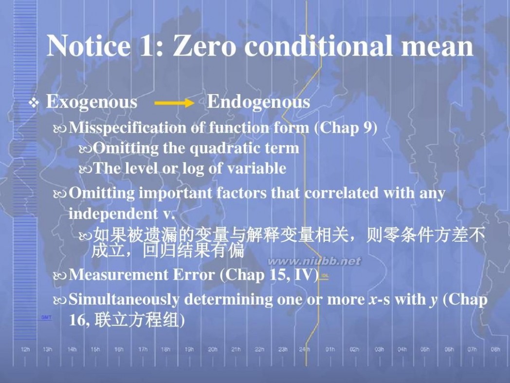
Notice 1: Zero conditional mean
Exogenous Endogenous
Misspecification of function form (Chap 9) Omitting the quadratic term The level or log of variable Omitting important factors that correlated with any independent v. 如果被遗漏的变量与解释变量相关, 如果被遗漏的变量与解释变量相关,则零条件方差不 成立, 成立,回归结果有偏 Measurement Error (Chap 15, IV) Simultaneously determining one or more x-s with y (Chap 16, 联立方程组 联立方程组)
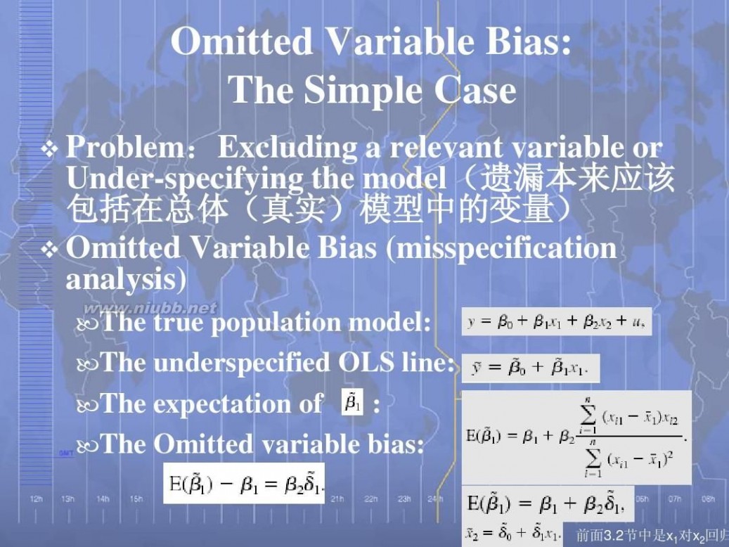
Omitted Variable Bias: The Simple Case
Problem:Excluding a relevant variable or : Under-specifying the model(遗漏本来应该 ( 包括在总体(真实)模型中的变量) 包括在总体(真实)模型中的变量) Omitted Variable Bias (misspecification analysis)
The true population model: The underspecified OLS line: The expectation of : The Omitted variable bias:
前面3.2节中是x1对x2回归
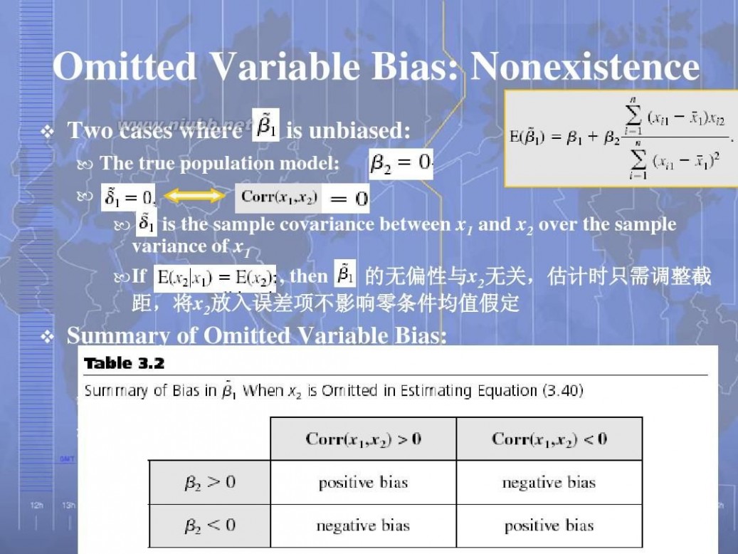
Omitted Variable Bias: Nonexistence
Two cases where is unbiased:
The true population model: is the sample covariance between x1 and x2 over the sample variance of x1 If , then 的无偏性与x 无关, 的无偏性与 2无关,估计时只需调整截 距,将x2放入误差项不影响零条件均值假定
Summary of Omitted Variable Bias:
The expectation of :
The Omitted variable bias:
The Size of Omitted Variable Bias
Direction Size A small bias of either sign need not be a cause for concern. Unknown Some idea
we usually have a pretty good idea about the direction of the partial effect of x2 on y, that is, the sign of in many cases we can make an educated guess about whether x1 and x2 are positively or negatively correlated.
E.g. (Upward/downward Bias; biased toward zero)
高估! 高估!
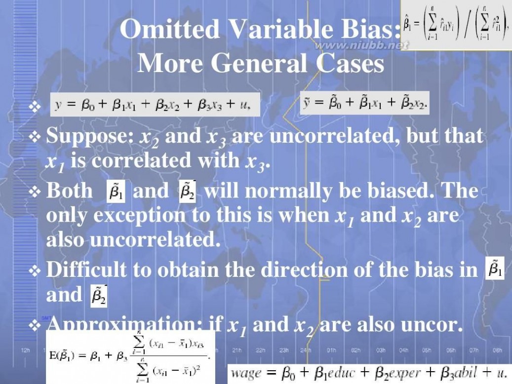
Omitted Variable Bias: More General Cases
Suppose: x2 and x3 are uncorrelated, but that x1 is correlated with x3. Both and will normally be biased. The only exception to this is when x1 and x2 are also uncorrelated. Difficult to obtain the direction of the bi
as in and Approximation: if x1 and x2 are also uncor.
Notice 2: No Perfect Collinearity
An assumption only about x-s, nothing about the relationship between u and x-s Assumption MLR.4 does allow the independent variables to be correlated; they just cannot be perfectly correlated. Ceteris Paribus effect
If we did not allow for any correlation among the independent variables, then multiple regression would not be very useful for econometric analysis. Significance
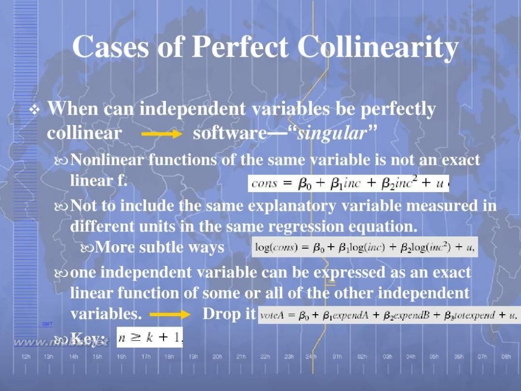
Cases of Perfect Collinearity
When can independent variables be perfectly collinear software—“singular”
Nonlinear functions of the same variable is not an exact linear f. Not to include the same explanatory variable measured in different units in the same regression equation. More subtle ways one independent variable can be expressed as an exact linear function of some or all of the other independent variables. Drop it Key:
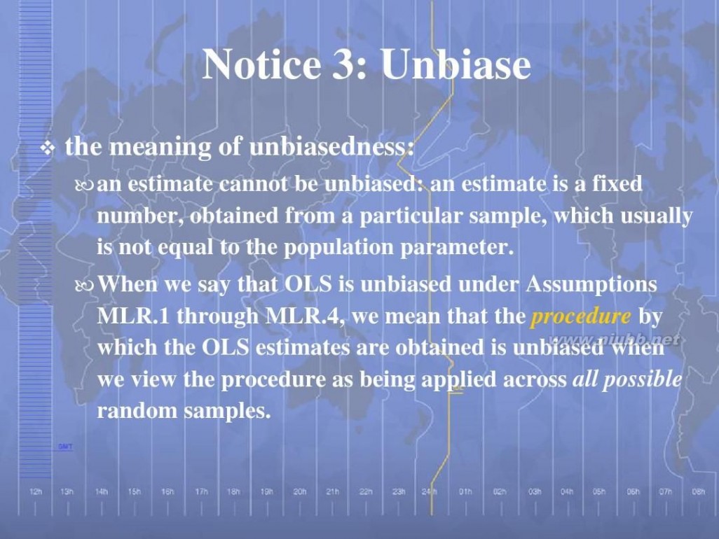
Notice 3: Unbiase
the meaning of unbiasedness:
an estimate cannot be unbiased: an estimate is a fixed number, obtained from a particular sample, which usually is not equal to the population parameter. When we say that OLS is unbiased under Assumptions MLR.1 through MLR.4, we mean that the procedure by which the OLS estimates are obtained is unbiased when we view the procedure as being applied across all possible random samples.
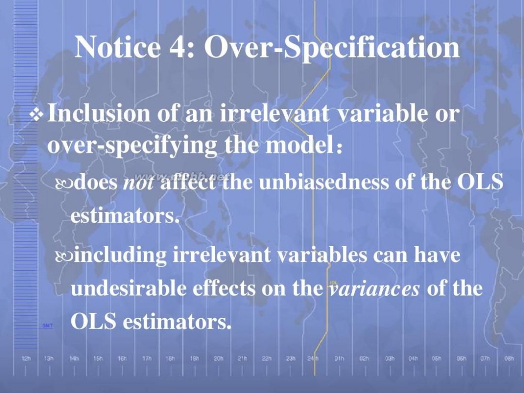
Notice 4: Over-Specification
Inclusion of an irrelevant variable or over-specifying the model: :
does not affect the unbiasedness of the OLS estimators. including irrelevant variables can have undesirable effects on the variances of the OLS estimators.
Variance of The OLS Estimators
Adding Assumptions
Homoskedasticity: Error variance A larger means that the distribution of the unobservables affecting y is more spread out.
Gauss-Markov assumptions (for cross-sectional regression): Assumption 1-5 Theorem (Sampling variance of OLS estimators)
Under the five assumptions above:
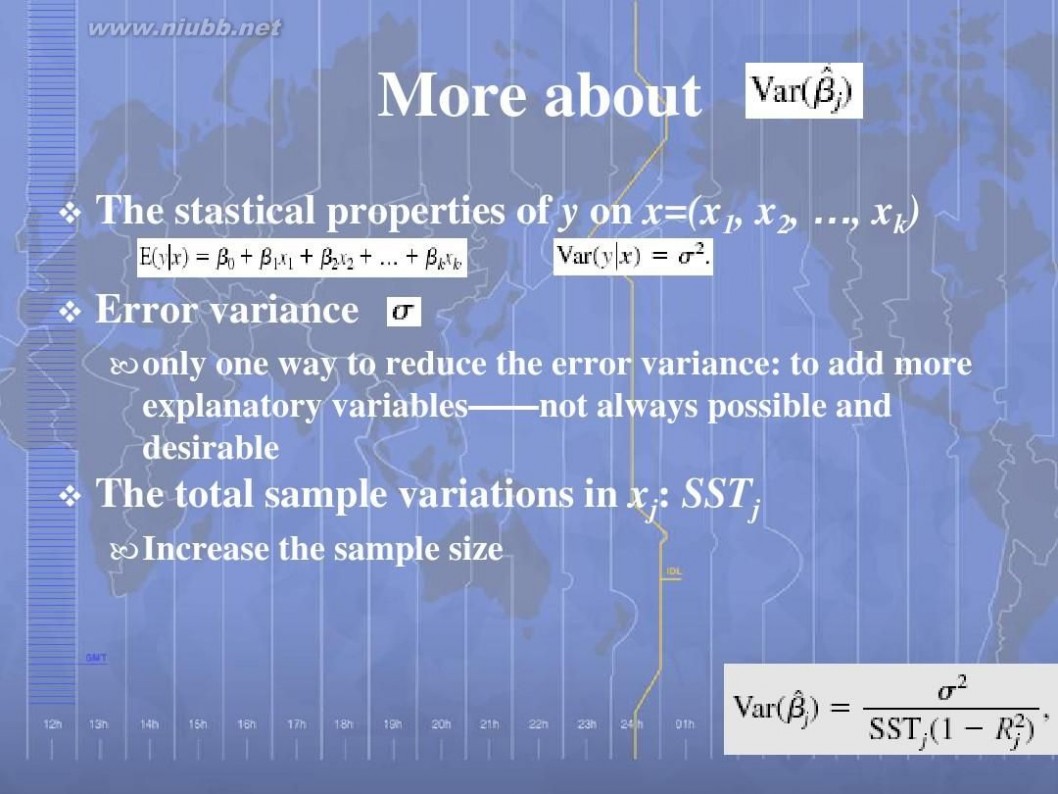
More about
The stastical properties of y on x=(x1, x2, …, xk) Error variance
only one way to reduce the error variance: to add more explanatory variables——not always possible and desirable
The total sample variations in xj: SSTj
Increase the sample size
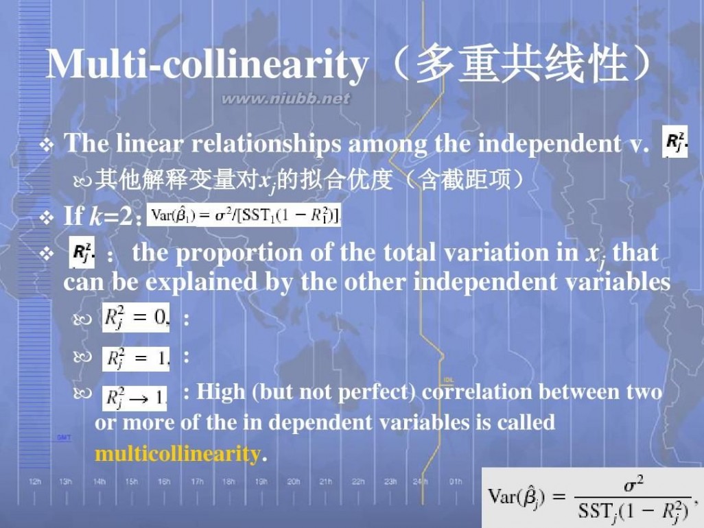
Multi-collinearity(多重共线性) (多重共线性)
The linear relationships among the independent v.
其他解释变量对x 的拟合优度(含截距项) 其他解释变量对 j的拟合优度(含截距项)
If k=2: : :the proportion of the total variation in xj that can be explained by the other independent variables
: : : High (but not perfect) correlation between two or more of the in dependent variables is called multicollinearity.
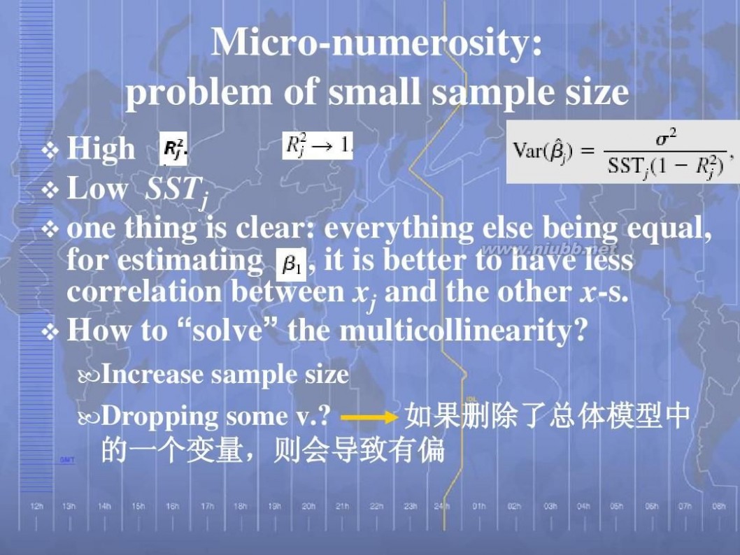
Micro-numerosity: problem of small sample size
High Low SSTj one thing is clear: everything else being equal, for estimating it is better to have less j, correlation between xj and the other x-s. How to “solve” the multicollinearity?
Increase sample size Dropping some v.? 如果删除了总体模型中 的一个变量, 的一个变
量,则会导致有偏
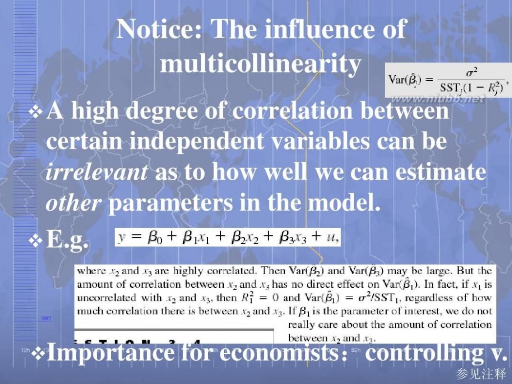
Notice: The influence of multicollinearity
A high degree of correlation between certain independent variables can be irrelevant as to how well we can estimate other parameters in the model. E.g.
Importance for economists:controlling v. :
参见注释
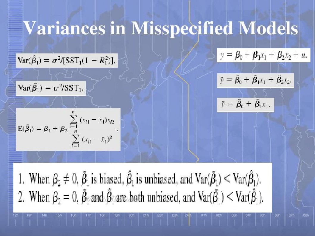
Variances in Misspecified Models
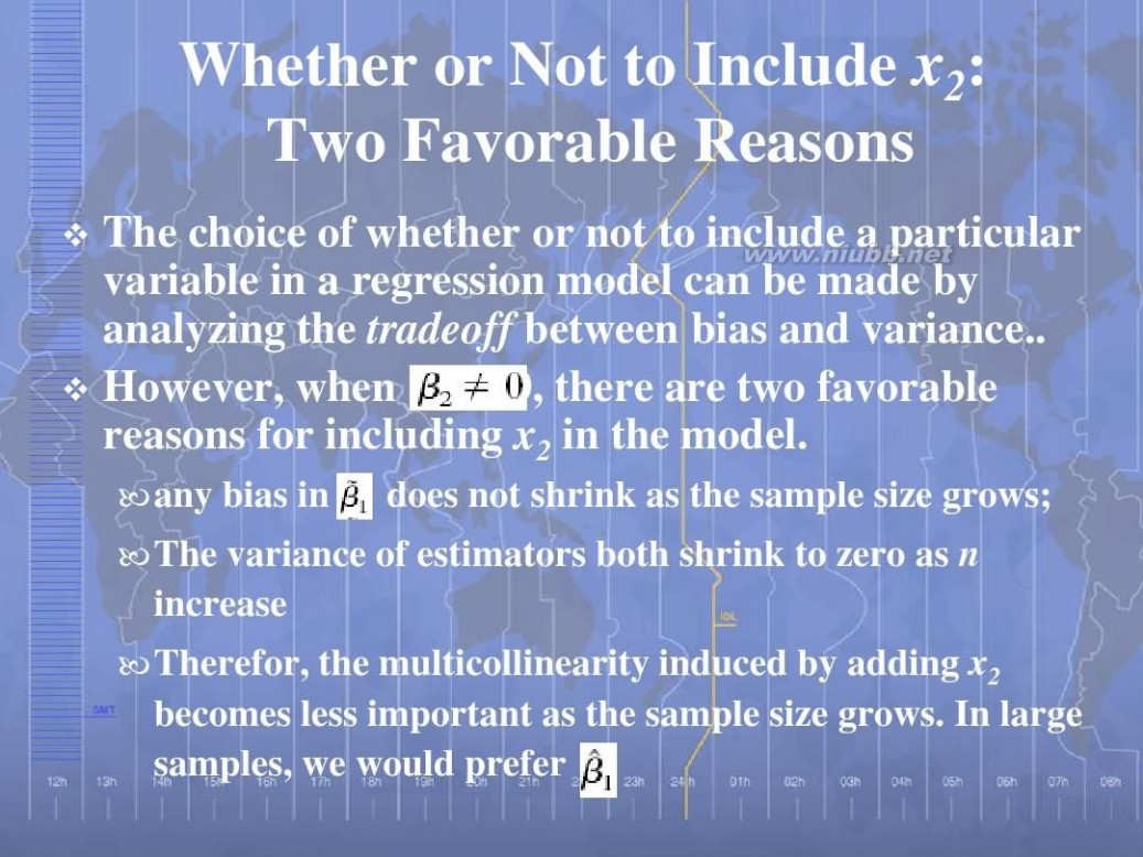
Whether or Not to Include x2: Two Favorable Reasons
The choice of whether or not to include a particular variable in a regression model can be made by analyzing the tradeoff between bias and variance.. However, when 0, there are two favorable 2 reasons for including x2 in the model.
any bias in does not shrink as the sample size grows; The variance of estimators both shrink to zero as n increase Therefor, the multicollinearity induced by adding x2 becomes less important as the sample size grows. In large samples, we would prefer
Estimating : Standard Errors of the OLS Estimators
参见 注释
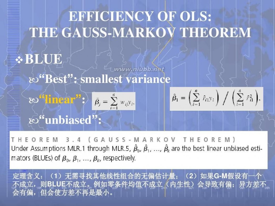
EFFICIENCY OF OLS: THE GAUSS-MARKOV THEOREM BLUE
“Best”: smallest variance “linear”: “unbiased”:
定理含义:( )无需寻找其他线性组合的无偏估计量;( ;(2)如果G-M假设有一个 定理含义:(1)无需寻找其他线性组合的无偏估计量;( )如果 :( 假设有一个 不成立, 不成立。 不成立,则BLUE不成立。例如零条件均值不成立(内生性)会导致有偏;异方差不 不成立 例如零条件均值不成立(内生性)会导致有偏; 会有偏,但会使方差不再是最小。 会有偏,但会使方差不再是最小。
Classical Linear Model Assumptions ——Inference
本部分课程内容参考资料
Jeffrey M. Wooldridge, Introductory Econometrics——A Modern Approach, Chap 2-3.
四 : MATLAB插值与拟合
实例:温度曲线问题
气象部门观测到一天某些时刻的温度变化数据为:
t | 0 | 1 | 2 | 3 | 4 | 5 | 6 | 7 | 8 | 9 | 10 |
T | 13 | 15 | 17 | 14 | 16 | 19 | 26 | 24 | 26 | 27 | 29 |
试描绘出温度变化曲线。
曲线拟合就是计算出两组数据之间的1种函数关系,由此可描绘其变化曲线及估计非采集数据对应的变量信息。
曲线拟合有多种方式,下面是一元函数采用最小二乘法对给定数据进行多项式曲线拟合,最后给出拟合的多项式系数。
1.线性拟合函数:regress()
调用格式: b=regress(y,X)
[b,bint,r,rint,stats]= regress(y,X)
[b,bint,r,rint,stats]= regress(y,X,alpha)
说明:b=regress(y,X)返回X处y的最小二乘拟合值。该函数求解线性模型:
y=Xβ+ε
β是p´1的参数向量;ε是服从标准正态分布的随机干扰的n´1的向量;y为n´1的向量;X为n´p矩阵。
bint返回β的95%的置信区间。r中为形状残差,rint中返回每1个残差的95%置信区间。Stats向量包含R2统计量、回归的F值和p值。
例1:设y的值为给定的x的线性函数加服从标准正态分布的随机干扰值得到。即y=10+x+ε;求线性拟合方程系数。
程序: x=[ones(10,1) (1:10)’]
y=x*[10;1]+normrnd(0,0.1,10,1)
[b,bint]=regress(y,x,0.05)
结果: x =
11
12
13
14
15
16
17
18
19
1 10
y =
10.9567
11.8334
13.0125
14.0288
14.8854
16.1191
17.1189
17.9962
19.0327
20.0175
b =
9.9213
1.0143
bint =
9.7889 10.0537
0.99301.0357
即回归方程为:y=9.9213+1.0143x
2.多项式曲线拟合函数:polyfit( )
调用格式: p=polyfit(x,y,n)
[p,s]= polyfit(x,y,n)
说明:x,y为数据点,n为多项式阶数,返回p为幂次从高到低的多项式系数向量p。矩阵s用于生成预测值的误差估计。(见下一函数polyval)
例2:由离散数据
x | 0 | .1 | .2 | .3 | .4 | .5 | .6 | .7 | .8 | .9 | 1 |
y | .3 | .5 | 1 | 1.4 | 1.6 | 1.9 | .6 | .4 | .8 | 1.5 | 2 |
拟合出多项式。
程序:
x=0:.1:1;
y=[.3 .5 1 1.4 1.6 1.9 .6 .4 .8 1.5 2]
n=3;
p=polyfit(x,y,n)
xi=linspace(0,1,100);
z=polyval(p,xi); %多项式求值
plot(x,y,’o’,xi,z,’k:’,x,y,’b’)
legend(‘原始数据’,’3阶曲线’)
结果:
p =
16.7832-25.745910.9802 -0.0035
多项式为:16.7832x3-25.7459x2+10.9802x-0.0035
曲线拟合图形:
也可由函数给出数据。
例3:x=1:20,y=x+3*sin(x)
程序:
x=1:20;
y=x+3*sin(x);
p=polyfit(x,y,6)
xi=1inspace(1,20,100);
z=poyval(p,xi);%多项式求值函数
plot(x,y,’o’,xi,z,’k:’,x,y,’b’)
legend(‘原始数据’,’6阶曲线’)
结果:
p =
0.0000-0.00210.0505-0.59713.6472-9.729511.3304

再用10阶多项式拟合
程序:x=1:20;
y=x+3*sin(x);
p=polyfit(x,y,10)
xi=linspace(1,20,100);
z=polyval(p,xi);
plot(x,y,'o',xi,z,'k:',x,y,'b')
legend('原始数据','10阶多项式')
结果:p =
Columns 1 through 7
0.0000-0.00000.0004-0.01140.1814-1.8065 11.2360
Columns 8 through 11
-42.086188.5907-92.8155 40.2671
可用不同阶的多项式来拟合数据,但也不是阶数越高拟合的越好。
3.多项式曲线求值函数:polyval( )
调用格式: y=polyval(p,x)
[y,DELTA]=polyval(p,x,s)
说明:y=polyval(p,x)为返回对应自变量x在给定系数P的多项式的值。
[y,DELTA]=polyval(p,x,s) 使用polyfit函数的选项输出s得出误差估计YDELTA。它假设polyfit函数数据输入的误差是独立正态的,并且方差为常数。则Y DELTA将至少包含50%的预测值。
4.多项式曲线拟合的评价和置信区间函数:polyconf( )
调用格式: [Y,DELTA]=polyconf(p,x,s)
[Y,DELTA]=polyconf(p,x,s,alpha)
说明:[Y,DELTA]=polyconf(p,x,s)使用polyfit函数的选项输出s给出Y的95%置信区间YDELTA。它假设polyfit函数数据输入的误差是独立正态的,并且方差为常数。1-alpha为置信度。
例4:给出上面例1的预测值及置信度为90%的置信区间。
程序:x=0:.1:1;
y=[.3 .5 1 1.4 1.6 1.9 .6 .4 .8 1.5 2]
n=3;
[p,s]=polyfit(x,y,n)
alpha=0.05;
[Y,DELTA]=polyconf(p,x,s,alpha)
结果: p =
16.7832-25.745910.9802 -0.0035
s =
df: 7
normr: 1.1406
Y =
Columns 1 through 7
-0.00350.85381.29701.42661.34341.14800.9413
Columns 8 through 11
0.82380.89631.25942.0140
DELTA =
Columns 1 through 7
1.36391.15631.15631.15891.13521.12021.1352
Columns 8 through 11
1.15891.15631.15631.3639
5.稳健回归函数:robust( )
稳健回归是指此回归方法相对于其他回归方法而言,受异常值的影响较小。
调用格式: b=robustfit(x,y)
[b,stats]=robustfit(x,y)
[b,stats]=robustfit(x,y,’wfun’,tune,’const’)
说明:b返回系数估计向量;stats返回各种参数估计;’wfun’指定1个加权函数;tune为调协常数;’const’的值为’on’(默认值)时添加1个常数项;为’off’时忽略常数项。
例5:演示1个异常数据点如何影响最小二乘拟合值与稳健拟合。首先利用函数y=10-2x加上一些随机干扰的项生成数据集,然后改变1个y的值形成异常值。调用不同的拟合函数,通过图形观查影响程度。
程序:x=(1:10)’;
y=10-2*x+randn(10,1);
y(10)=0;
bls=regress(y,[ones(10,1) x]) %线性拟合
brob=robustfit(x,y) %稳健拟合
scatter(x,y)
hold on
plot(x,bls(1)+bls(2)*x,’:’)
plot(x,brob(1)+brob(2)*x,’r‘)
结果 : bls =
8.4452
-1.4784
brob =
10.2934
-2.0006
分析:稳健拟合(实线)对数据的拟合程度好些,忽略了异常值。最小二乘拟合(点线)则受到异常值的影响,向异常值偏移。
6.向自定义函数拟合
对于给定的数据,根据经验拟合为带有待定常数的自定义函数。
所用函数:nlinfit( )
调用格式:[beta,r,J]=nlinfit(X,y,’fun’,betao)
说明:beta返回函数’fun’中的待定常数;r表示残差;J表示雅可比矩阵。X,y为数据;‘fun’自定义函数;beta0待定常数初值。
例6:在化工生产中获得的氯气的级分y随生产时间x下降,假定在x≥8时,y与x之间有如下形式的非线性模型:
现收集了44组数据,利用该数据通过拟合确定非线性模型中的待定常数。
xyxyxy
80.49160.43280.41
80.49180.46280.40
100.48180.45300.40
100.47200.42300.40
100.48200.42300.38
100.47200.43320.41
120.46200.41320.40
120.46220.41340.40
120.45220.40360.41
120.43240.42360.36
140.45240.40380.40
140.43240.40380.40
140.43260.41400.36
160.44260.40420.39
160.43260.41
首先定义非线性函数的m文件:fff6.m
function yy=model(beta0,x)
a=beta0(1);
b=beta0(2);
yy=a+(0.49-a)*exp(-b*(x-8));
程序:
x=[8.00 8.00 10.00 10.00 10.00 10.0[www.61k.com)0 12.00 12.00 12.00 14.0014.00 14.00...
16.00 16.00 16.00 18.00 18.00 20.00 20.00 20.00 20.00 22.00 22.0024.00...
24.00 24.00 26.00 26.00 26.00 28.00 28.00 30.00 30.00 30.00 32.0032.00...
34.00 36.00 36.00 38.00 38.00 40.00 42.00]';
y=[0.49 0.49 0.48 0.470.48 0.47 0.46 0.46 0.45 0.43 0.45 0.43 0.43 0.44 0.43...
0.43 0.46 0.42 0.42 0.43 0.41 0.41 0.40 0.42 0.40 0.40 0.41 0.400.41 0.41...
0.40 0.40 0.40 0.38 0.41 0.40 0.40 0.41 0.38 0.40 0.40 0.390.39]';
beta0=[0.30 0.02];
betafit = nlinfit(x,y,'sta67_1m',beta0)
结果:betafit =
0.3896
0.1011
即:a=0.3896 ,b=0.1011 拟合函数为:
在应用领域中,由有限个已知数据点,构造1个解析表达式,由此计算数据点之间的函数值,称之为插值。
实例:海底探测问题
某公司用声纳对海底进行测试,在5×5海里的坐标点上测得海底深度的值,希望通过这些有限的数据悉更多处的海底情况。并绘出较细致的海底曲面图。
一、一元插值
一元插值是对一元数据点(xi,yi)进行插值。
1.线性插值:由已知数据点连成一条折线,认为相临2个数据点之间的函数值就在这两点之间的连线上。一般来说,数据点数越多,线性插值就越精确。
调用格式:yi=interp1(x,y,xi,’linear’)%线性插值
zi=interp1(x,y,xi,’spline’) %三次样条插值
wi=interp1(x,y,xi,’cubic’) %三次多项式插值
说明:yi、zi、wi为对应xi的不同类型的插值。x、y为已知数据点。
例1:已知数据:
x | 0 | .1 | .2 | .3 | .4 | .5 | .6 | .7 | .8 | .9 | 1 |
y | .3 | .5 | 1 | 1.4 | 1.6 | 1.9 | .6 | .4 | .8 | 1.5 | 2 |
求当xi=0.25时的yi的值。
程序:
x=0:.1:1;
y=[.3 .5 1 1.4 1.6 1 .6 .4 .8 1.5 2];
yi0=interp1(x,y,0.025,'linear')
xi=0:.02:1;
yi=interp1(x,y,xi,'linear');
zi=interp1(x,y,xi,'spline');
wi=interp1(x,y,xi,'cubic');
plot(x,y,'o',xi,yi,'r+',xi,zi,'g*',xi,wi,'k.-')
legend('原始点','线性点','三次样条','三次多项式')
结果:yi0 = 0.3500
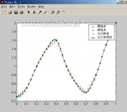
要得到给定的几个点的对应函数值,可用:
xi =[ 0.2500 0.35000.4500]
yi=interp1(x,y,xi,'spline')
结果:
yi =1.20881.5802 1.3454
(二) 二元插值
二元插值与一元插值的基本思想一致,对原始数据点(x,y,z)构造见世面函数求出插值点数据(xi,yi,zi)。
一、单调节点插值函数,即x,y向量是单调的。
调用格式1:zi=interp2(x,y,z,xi,yi,’linear’)
‘liner’ 是双线性插值 (缺省)
调用格式2:zi=interp2(x,y,z,xi,yi,’nearest’)
’nearest’ 是最近邻域插值
调用格式3:zi=interp2(x,y,z,xi,yi,’spline’)
‘spline’是三次样条插值
说明:这里x和y是2个独立的向量,它们必须是单调的。z是矩阵,是由x和y确定的点上的值。z和x,y之间的关系是z(i,:)=f(x,y(i))z(:,j)=f(x(j),y)即:当x变化时,z的第i行与y的第i个元素相关,当y变化时z的第j列与x的第j个元素相关。如果没有对x,y赋值,则默认x=1:n,y=1:m。n和m分别是矩阵z的行数和列数。
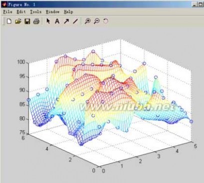
例2:已知某处山区地形选点测量坐标数据为:
x=0 0.51 1.5 22.5 3 3.54 4.5 5
y=0 0.51 1.5 22.5 3 3.54 4.5 55.5 6
海拔高度数据为:
z=89 90 87 85 92 91 96 93 90 87 82
92 96 98 99 9591 89 86 84 82 84
96 98 95 92 9088 85 84 83 81 85
80 81 82 89 9596 93 92 89 86 86
82 85 87 98 9996 97 88 85 82 83
82 85 89 94 9593 92 91 86 84 88
88 92 93 94 9589 87 86 83 81 92
92 96 97 98 9693 95 84 82 81 84
85 85 81 82 8080 81 85 90 93 95
84 86 81 98 9998 97 96 95 84 87
80 81 85 82 8384 87 90 95 86 88
80 82 81 84 8586 83 82 81 80 82
87 88 89 98 9997 96 98 94 92 87
其地貌图为:
对数据插值加密形成地貌图。
程序:
x=0:.5:5;
y=0:.5:6;
z=[89 90 87 85 92 91 96 93 90 87 82
92 96 98 9995 91 89 86 84 82 84
96 98 95 9290 88 85 84 83 81 85
80 81 82 8995 96 93 92 89 86 86
82 85 87 9899 96 97 88 85 82 83
82 85 89 9495 93 92 91 86 84 88
88 92 93 9495 89 87 86 83 81 92
92 96 97 9896 93 95 84 82 81 84
85 85 81 8280 80 81 85 90 93 95
84 86 81 9899 98 97 96 95 84 87
80 81 85 8283 84 87 90 95 86 88
80 82 81 8485 86 83 82 81 80 82
87 88 89 9899 97 96 98 94 92 87];
mesh(x,y,z) %绘原始数据图
xi=linspace(0,5,50);%加密横坐标数据到50个
yi=linspace(0,6,80);%加密纵坐标数据到60个
[xii,yii]=meshgrid(xi,yi);%生成网格数据
zii=interp2(x,y,z,xii,yii,'cubic');%插值
mesh(xii,yii,zii)%加密后的地貌图
holdon% 保持图形
[xx,yy]=meshgrid(x,y);%生成网格数据
plot3(xx,yy,z+0.1,’ob’)%原始数据用‘O’绘出
2、二元非等距插值
调用格式:zi=griddata(x,y,z,xi,yi,’指定插值方法’)
插值方法有:linear% 线性插值 (默认)
bilinear% 双线性插值
cubic% 三次插值
bicubic% 双三次插值
nearest% 最近邻域插值
例:用随机数据生成地貌图再进行插值
程序:
x=rand(100,1)*4-2;
y=rand(100,1)*4-2;
z=x.*exp(-x.^2-y.^2);
ti=-2:.25:2;
[xi,yi]=meshgrid(ti,ti); % 加密数据
zi=griddata(x,y,z,xi,yi);% 线性插值
mesh(xi,yi,zi)
hold on
plot3(x,y,z,'o')

该例中使用的数据是随机形成的,故函数griddata可以处理无规则的数据。
本文标题:插值与拟合-51插值与拟合例题61阅读| 精彩专题| 最新文章| 热门文章| 苏ICP备13036349号-1